For convenience, we will usually think of \( x \in \RR^n \) and \( a \in \ZZ^n \) and say that \( a \) is an integer realtion of \( x \).

Aside: picture proof that \( \arctan{1} + \arctan{2} + \arctan{3} = \pi \)
and so \( (4,-3,4) \) really is an integer relation for \( (\arctan{2}, \pi, \arctan{3}) \).

History

Euclid's extended algorithm.

• \( a\,m + b\,n = \gcd(a,b) \) relates \( a \), \( b \), and \( \gcd(a,b) \) by integers.
• Each iteration produces incrementally better approximation.
• Also works for real numbers (see Book X, Prop 3).

History

General case (for more than 2 numbers).

• Sought after by: Euler, Jacobi, Pincaré, Minkowski, Perron, Brun, Mahler, and others.
• None proved to work for \( n > 3 \)
• None adequately captured the increasing approximation property.

History

Generalisations satisfying both properties.

• First one published by Ferguson & Forcade in 1979 with extensive, unpublished notes, by Bergman.
• Several intermediate results (Ferguson & Forcade 1982, Ferguson 1986, Ferguson 1987).
• PSOS algorithm (Ferguson 1988)
• PSLQ algorithm (Ferguson & Bailey 1992)

Applications

Can see if a number \( \alpha \) satisfies an integer polynomial by searching for integer relations of \( (\alpha^0, \alpha^1, \dotsc, \alpha^n) \)

Bailey & Ferguson used such a technique to show \( \gamma, \log\gamma, \log\pi, \zeta(3) \) and some others do not satisfy a low-degree polynomial.

Applications

Borwein Bailey Plouffe formula \[ \pi =\sum_{k=0}^\infty \left( \frac{1}{16^k} \left( \frac{4}{8k+1} - \frac{2}{8k+4} - \frac{1}{8k+5} - \frac{1}{8k+6} \right)\right)\] found by “inspired guessing and extensive searching using the PSLQ integer relation algorithm”

Applications

Bailey & Plouffe use PSLQ to search for (“recognise”) symbolic representations of floating point numbers.

E.g., they were able to recognise that \[ 1.6083594219855456\dotso \approx \int_{0}^\infty t^{7/4}\,e^{-t}\,\mathrm{d}t = \frac{21\pi\sqrt{2}}{16\,\Gamma(1/4)} \] (note that the RHS can be reduced to \(\frac{21}{16} \, \Gamma(3/4) \))

Applications

Chamberland uses PSLQ to find relationships between functions.

There are many others. See Borwein & Lisoněk 2000 “Applications of Integer Relation Algorithms” (DOI: 10.1016/S0012-365X(99) 00256-3).

We can extend the idea to allow complex numbers.

Note that \( \ZZ[i] = \left\{ a + bi: a,b \in \ZZ \right\} \)

This definition encapsulates the previous one.

When talking about integer relations in general, we use the following notation so as to encapsulate all cases.

The classical cases, then, are when \( \mathcal{O} = \ZZ \) and \( \FF = \RR\), and when \( \mathcal{O} = \ZZ[i] \) and \( \FF = \CC \).

We will sometimes refer to an \( \mathcal{O} \)-lattice if we need to specify the integer ring explicitly.

We can represent a lattice \( L \) as a matrix by using the basis vectors as row vectors.

Note that the literature often uses column vectors instead of row vectors.

An information theoretic argument shows that in order to numerically compute an integer relation on \( n \) numbers, where the relation consists of integers with no more than \( d \) digits, then at least \( nd \) decimal digits of precision need to be used.

In the case of complex numbers and Gaussian integers, the number of digits is the number of digits in the real part, or the imaginary part, whichever is larger.

LLL

The LLL algorithm was introduced by Lenstra, Lenstra Jr, and Lovasz in 1982.

It is not an algorithm for computing integer relations directly. Instead it finds short lattice vectors

It can, however, be used to compute integer relations

LLL

Given a basis \( B \) for a lattice \( L \), the LLL algorithm computes a basis \( B^\prime = (b^\prime_1,\dotsc,b^\prime_n) \) such that \[ \begin{gather} \lvert \mu_{i,j} \rvert \le \frac{1}{2} \text{ for } 1 \le j < i \le n \\ \lvert\lvert b^*_i + \mu_{i,j} b^*_{i-1} \rvert\rvert^2 \ge \frac{3}{4} \lvert\lvert b^*_{i-1} \rvert\rvert^2 \text{ for } 1 < i \le n \\ \end{gather} \] where \( b^*_i = b^\prime_i - \sum_{j=1}^{i-1}\mu_{i,j}b^*_j \text{ and } \mu_{i,j} = \frac{ b^\prime_i \cdot b^*_j}{\lvert\lvert b^*_j \rvert\rvert^2} \)

LLL

To find an integer relation on \( x = (x_1, \dotsc, x_n) \in \RR^n \) we can use LLL on the lattice \[ L := \begin{bmatrix} 1 & 0 & 0 & \dotsm & 0 & Nx_1 \\ 0 & 1 & 0 & \dotsm & 0 & Nx_2 \\ \vdots & \vdots & \ddots & \dotsm & \vdots & \vdots \\ 0 & 0 & 0 & \dotsm & 1 & Nx_n \end{bmatrix}\] for some \( N \in \RR \).

Think of this as the augmented matrix \( \left[ I_n\, Nx \right] \).

LLL

Elements of the lattice look like \[ \left(\lambda_1, \dotsc, \lambda_n, N(\lambda_1x_1 + \dotsm + \lambda_nx_n) \right) \] So if the \( \lambda_i \) are an integer relation for \( x \) then the last term will be 0.

We can prove that if \( N \) is large enough, then the first element of the reduced lattice must contain the integer relation.

LLL

For the complex case where n \( z = (z_1, \dotsc, z_n) \in \CC^n \) we still use the augmented lattice \( L := \left[ I_n \, Nz \right] \) like we did for the real case.

However we then construct a 2nd augmented lattice \[ \begin{bmatrix} \Re{L} & \Im{L} \\ -\Im{L} & \Re{L}\end{bmatrix} \] and use LLL on that lattice.

As with the real case, so long as \( N \) is large enough then the procedure must find an integer relation.

LLL

In all cases, we don't know how large to make \( N \) before we start. So we must use trial and error.

We have found, experimentally, that with numeric (floating point) calculations it is possible for \( N \) to be too large, even though the theory requires \( N \) to be “sufficiently large”.

PSLQ

The PSLQ algorithm was introduced by Ferguson & Bailey in 1988. It was later analysed by Ferguson, Bailey, and Arno in 1999

It can handle both the real and complex cases directly.

We will not discuss the details of the algorithm itself. However we will establish some facts.

PSLQ

Observe that in both the real and complex cases \( \mathcal{O} \) forms a lattice, and that \( \mathcal{O} \subset \FF \).

We denote by \( \lceil \cdot \rfloor_{\mathcal{O}} \) if we need to be specific.

PSLQ

There are parameters: \( \gamma, \rho \), and \( \tau \) that must satisfy \[ \begin{gather} \frac{1}{\rho} \ge \lvert x - \lceil x \rfloor \rvert \text{ for all } x \in \FF \\ 1 \le \tau \le \rho \\ \frac{1}{\tau^2} = \frac{1}{\gamma^2} + \frac{1}{\rho^2} \end{gather} \]

\( \rho \) is bounded by the integer lattice; choose to maximise \(1/\rho\).

\( \gamma \) is minimised when \( \tau = 1 \); choose any larger value.

\( \tau \) is fixed by the choice of \( \gamma \) and the value of \( \rho \).

PSLQ

Each iteration of the PSLQ algorithm finds an increased lower bound on the norm of any integer relation on the input.

The algorithm can terminate when that bound exceeds some threshold.

If the algorithm finds a relation, \( a \) then \( \lvert\lvert a \rvert\rvert \le \gamma^{n-2}M \) where \( M \) is the norm of the smallest possible relation.

Comparing LLL and PSLQ

LLL requires more precision than PSLQ

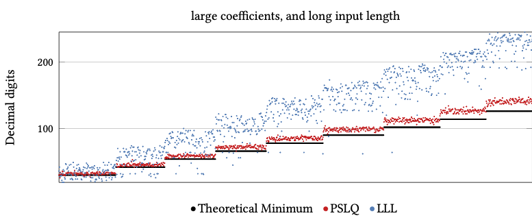
Real Integer Relation Problems

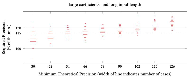
Comparing LLL and PSLQ

LLL requires more precision than PSLQ

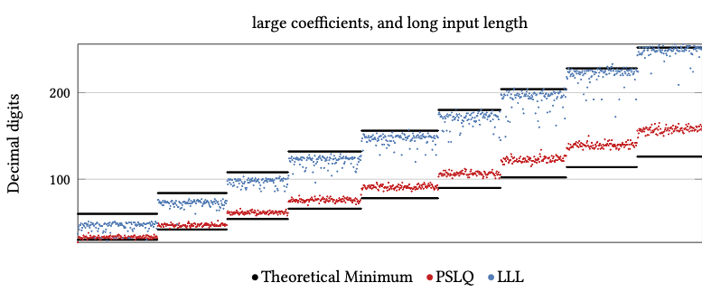
Complex Integer Relation Problems (real constants)

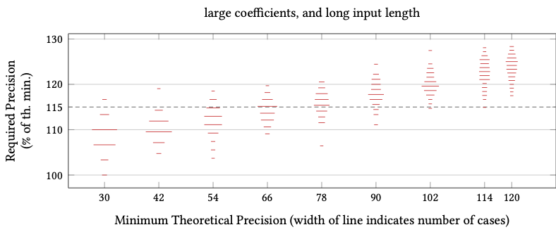
Comparing LLL and PSLQ

LLL requires more precision than PSLQ

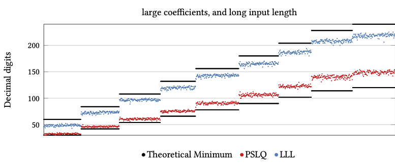
Complex Integer Relation Problems (complex constants)

Comparing LLL and PSLQ

PSLQ Required Precision (as % of theoretical min).

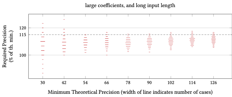
Real Integer Relation Problems

Comparing LLL and PSLQ

PSLQ Required Precision (as % of theoretical min).

Complex Integer Relation Problems (real constants)

Comparing LLL and PSLQ

PSLQ Required Precision (as % of theoretical min).

Complex Integer Relation Problems (complex constants)

Comparing LLL and PSLQ

LLL takes much more time than PSLQ

Real Integer Relation Problems

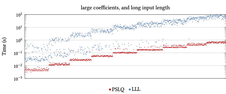
Comparing LLL and PSLQ

LLL takes much more time than PSLQ

Complex Integer Relation Problems (real constants)

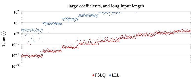
Comparing LLL and PSLQ

LLL takes much more time than PSLQ

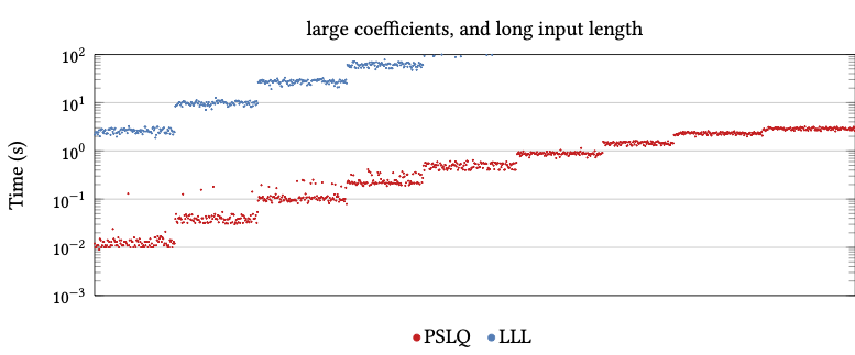
Complex Integer Relation Problems (complex constants)

Note that the literature often uses the notation \( \KK/\FF \) instead.

For example \( \sqrt{2} \) satisfies \( k^2 - 2 = 0 \) and so is algebraic over the rationals.

An integral domain is a commutative ring with multiplicative identity and no non-zero elements \( d_1, d_2 \) with the property that \( d_1d_2 = 0 \).

Note that the ring \( \ZZ \) is often called the “rational integers” to avoid ambiguity.

We are primarily interested in extension fields of \( \QQ \).

An algebraic extension is real if \( \KK \subseteq \RR \) and complex otherwise.

We are primarily interested in extension fields of \( \QQ \).

We are primarily interested in extension fields of \( \QQ \).

Quadratic Fields

We will restrict our attention to quadratic extension fields. These are fields of the form: \[ \QQ( \sqrt{D} ) = \left\{ q_1 + q_2 \sqrt{D} : q_i \in \QQ \right\} \] wher \( D \in \ZZ \) is square free.

Elements of these fields satisfy quadratic (or lower degree) polynomials with rational coefficients.

Quadratic Fields

The algebraic integers of a quadratic field (which we call quadratic integers) are of the form \[ \mathcal{O}_{\QQ(\sqrt{D})} = \ZZ[\omega] = \left\{ m_1 + m_2 \omega : m_i \in \mathbb{Z} \right\} \] where \[ \omega = \begin{cases} \sqrt{D} & \text{ if } D \equiv 2,3 \;(\operatorname{mod} 4) \\ \frac{1+\sqrt{D}}{2} & \text{ if } D \equiv 1 \;(\operatorname{mod} 4) \end{cases} \]

Quadratic Fields

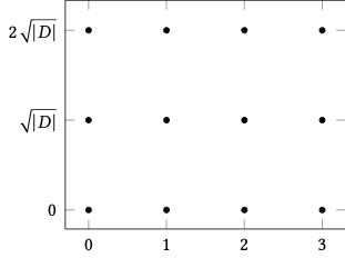
\( D \equiv 2,3 \;(\operatorname{mod} 4) \)

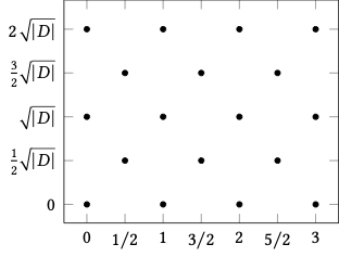
\( D \equiv 1 \;(\operatorname{mod} 4) \)

Quadratic Fields

Finally we mention a special class of quadratic fields.

Relations With Algebraic Integers

Recall the definiton of an integer relation:

Relations With Algebraic Integers

We could try and replace \( \CC \) with an algebraic extension field, and replace \( \ZZ[i] \) with the ring of integers of that field.

However, this won't capture the existing cases.

Relations With Algebraic Integers

We could try and replace \( \CC \) with an algebraic extension field, and replace \( \ZZ[i] \) with the ring of integers of that field.

However, this won't capture the existing cases.

The fields \( \RR \) and \( \CC \) are not algebraic fields (although they are extension fields of \( \QQ \) ). Thus they do not have algebraic integers.

If we try to take the intersections anyway (\( \RR \cap \mathcal{A} \) or \( \CC \cap \mathcal{A} \)) we do not get correct integers.

Relations With Algebraic Integers

Instead, specify an intermediate extension field.

Reduction to Classical Cases

Observe that for an quadratic integer relation: \[ \begin{align*} & \left(m_{1,1} + m_{1,2} \omega\right)\,x_1 + \dotsm + \left(m_{n,1} + m_{n,2}\omega\right)\,x_n \\ =& \left(m_{1,1}x_1 + \dotsm + m_{n,1}x_n \right) + \left(m_{1,2}\, \omega x_1 + \dotsm m_{n,2}\,\omega x_n\right) \end{align*} \]

This suggests a way to reduce a quadratic integer relation to a classical one.

Reduction to Classical Cases

Given \( (x_1, \dotsc, x_n) \in \FF^n \) we compute \( (x_1, \dotsc, x_n, x_1\omega, \dotsc, x_n\omega) \in \FF^{2n} \) and search for a classical integer relation on that.

We recover the integer relation by taking \( a_k + a_{n+k}\omega \) for \( 1 \le k \le n \).

This works well for real quadratic fields (i.e., when \( D > 1 \)). It works less well for complex quadratic fields.

Reduction to Classical Cases

In the complex case, the integers are of the form \( a_k = m_{k,1} + m_{k,2} i \). So when we attempt to recover the relation we get \[ \left(m_{k,1} + m_{k,2} i\right) + \left(m_{k+n,1} + m_{k+n,2} i \right)\omega \] after expansion and some simplification we get \[ \alpha_1 + \beta_2 i \sqrt{\lvert D \rvert} + \alpha_2 i - \beta_2 \sqrt{\lvert D \rvert} \text{ for } \alpha_1, \beta_1 \in \ZZ \] which is not an algebraic integer in \( \QQ(\sqrt{D}) \) if \( \alpha_2 \ne 0 \) or \( \beta_2 \ne 0 \).

Reduction to Classical Cases

Much of the time the reduction technique works fine, and gives good answers even in the complex cases.

When it does not work, we try two techniques to nonetheless extract a relation.

Reduction to Classical Cases

Decomposition method

We observe that \[ \alpha_1 + \beta_2 i \sqrt{\lvert D \rvert} + \alpha_2 i - \beta_2 \sqrt{\lvert D \rvert}\] can be written as \[ \left( \alpha_1 + \beta_2 i\sqrt{\lvert D \rvert} \right) + i \left( \alpha_2 + \beta_2 \sqrt{\lvert D \rvert} \right) \] and we have two possible algebraic integers embedded. We try extracting only these.

Reduction to Classical Cases

Conjugate Method

Given \[ \alpha_1 + \beta_2 i \sqrt{\lvert D \rvert} + \alpha_2 i - \beta_2 \sqrt{\lvert D \rvert} \] a conjugate is \[ \alpha_1 - \beta_2 i \sqrt{\lvert D \rvert} - \alpha_2 i - \beta_2 \sqrt{\lvert D \rvert} \]

Multiplying the number by its conjugate gives an element of \( \mathcal{O}_{\QQ(\sqrt{D})} \). We multiply all elements of the relation by the conjugate of only one of the elements.

Reduction to Classical Cases

Both the methods for correcting the complex case work well in practice.

We do not have proofs that they will always be correct. It is nonetheless easy to just try them, and check the extracted relation.

Using LLL

To compute an algebraic integer n \( z = (z_1, \dotsc, z_n) \in \FF^n \) we still use the augmented lattice \( L := \left[ I_n \, Nz \right] \) like we did for the real case.

However we then construct a 2nd augmented lattice. \[ \begin{bmatrix} \Re{L} & \Im{L} \\ \mathfrak{W_1}{L} & \mathfrak{W_2}{L}\end{bmatrix} \] and use LLL on that lattice.

Using LLL

However we then construct a 2nd augmented lattice. \[ \begin{bmatrix} \Re{L} & \Im{L} \\ \mathfrak{W_1}{L} & \mathfrak{W_2}{L}\end{bmatrix} \] and use LLL on that lattice.

\[ \mathfrak{W_1}{x_k} = \begin{cases} -\sqrt{\lvert D \rvert} \Im{x_k} & \text{ if } \text{ if } D \equiv 2,3 \;(\operatorname{mod} 4) \\ \left(\Re{x_k} - \sqrt{\lvert D \rvert}\Im{x_k} \right)/2 & \text{ if } D \equiv 1 \;(\operatorname{mod} 4) \end{cases} \] \[ \mathfrak{W_1}{x_k} = \begin{cases} -\sqrt{\lvert D \rvert} \Im{x_k} & \text{ if } \text{ if } D \equiv 2,3 \;(\operatorname{mod} 4) \\ \left(\Re{x_k} - \sqrt{\lvert D \rvert}\Im{x_k} \right)/2 & \text{ if } D \equiv 1 \;(\operatorname{mod} 4) \end{cases} \]

Using LLL

As with the other cases, so long as \( N \) is large enough then the procedure must find an algebraic integer relation.

Modifying PSLQ

We attempt to modify PSLQ while keeping the existing theory.

We simply use a quadratic integer nearest integer function, and modify the algorithm to allow us to specify the quadratic extension field we wish to use.

Modifying PSLQ

We simply use a quadratic integer nearest integer function, and modify the algorithm to allow us to specify the quadratic extension field we wish to use.

This introduces a problem: for real quadratic extension fields, the integers do not form a lattice (there is no unique nearest integer to a field element), so we cannot use the existing theory.

We restrict our attention to the complex cases, then.

Modifying PSLQ

We restrict our attention to the complex cases, then.

In these cases we have a more subtle problem.

As \( D \) increases, the parameter \( \rho \) decreases, until eventually \( \rho < 1 \) making it impossible to satisfy the \( 1 < \tau \le \rho \) condition.

Modifying PSLQ

In these cases we have a more subtle problem.

As \( D \) increases, the parameter \( \rho \) decreases, until eventually \( \rho < 1 \) making it impossible to satisfy the \( 1 < \tau \le \rho \) condition.

The complex quadratic fields that do not exhibit these problems are exactly: \[ \QQ(\sqrt{-2}), \QQ(\sqrt{-3}), \QQ(\sqrt{-7}), \QQ(\sqrt{-11})\]

Modifying PSLQ

As \( D \) increases, the parameter \( \rho \) decreases, until eventually \( \rho < 1 \) making it impossible to satisfy the \( 1 < \tau \le \rho \) condition.

The complex quadratic fields that do not exhibit these problems are exactly: \[ \QQ(\sqrt{-2}), \QQ(\sqrt{-3}), \QQ(\sqrt{-7}), \QQ(\sqrt{-11})\]

These are precisely the complex quadratic norm Euclidean fields.

Modifying PSLQ

The complex quadratic fields that do not exhibit these problems are exactly: \[ \QQ(\sqrt{-2}), \QQ(\sqrt{-3}), \QQ(\sqrt{-7}), \QQ(\sqrt{-11}) \]

We note that we've had surprising success with the modified PSLQ on \[ \QQ(\sqrt{-5}), \QQ(\sqrt{-6}), \QQ(\sqrt{-10}) \] even though they do not fit the existing theory.